Anomaly Detection with Auto-Encoders

In data science, anomaly detection is when the system tries to detect a rare item, event or observation which deviates significantly from the original distribution and can not be defined as normal behaviour. Three different categories of anomaly detection exist:
- Supervised anomaly detection
- Semi-supervised anomaly detection
- Unsupervised anomaly detection
In this project, we will be using an unsupervised approach to detect the regions of the hazelnut images that do not match the distribution.
1. Background
1.1 Anomaly Detection
Anomaly detection, also known as out-layer analysis, is a step-in data mining that identifies data points, events, and observations that deviate from a data set’s normal behaviour. It is the process of finding patterns in data that do not conform to prior expected behaviour. Anomaly detection is being employed increasingly in the presence of big data that is captured by sensors, social media platforms, huge networks, etc. They also have many applications, including energy systems, medical devices, banking network intrusion detection, etc. Machine learning is progressively being used to automate anomaly detection.
1.2. Auto-Encoders
Auto Encoder is a generative unsupervised deep learning the algorithm used for reconstructing high-dimensional input data using a neural network with a narrow bottleneck layer in the middle that contains the latent representation of the input data. Auto-Encoders have two main parts called, Encoder and Decoder.
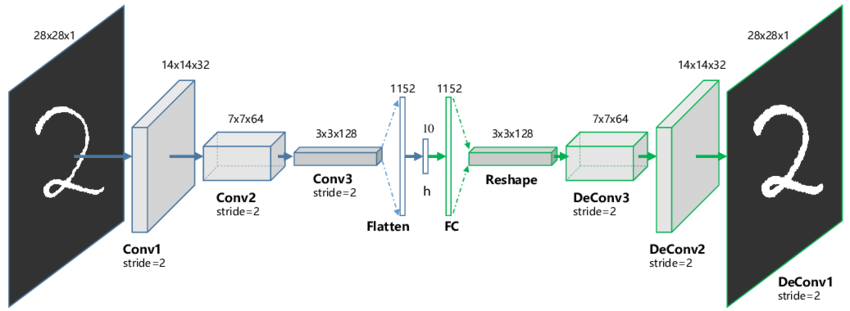
- Encoder: Accepts high-dimensional input data and translates it to latent low-dimensional data. The input size of an Encoder network is larger than its output size.
- Decoder: The Decoder network receives the input from the Encoder coder’s output. The Decoder’s objective is to reconstruct the input data. The output size of a Decoder network is larger than its input size.
1.3 Accuracy methods
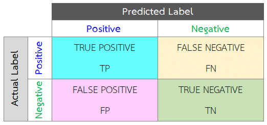
In order to be able to compare our results with those already published, we need to have a standard accuracy method. First off, we need to know the concept of True and Predicted conditions. Two types of correct predictions (True Positives and True Negatives), and there are two types of errors. Error Type I for any observation predicted positive when it is negative (False Positive, also called False Alert). Error Type II for any observation predicted negative when it is positive (False Negative).
2. Dataset
For our project, we used the MVTec dataset that belonged to Paul Bergmann, January 2021,this data set contained several different groups of images such as Bottles, Cables, Capsule, Carpet, Grid, Hazelnut, Leather, Metal Nut, Pill, Screw, Tile, Toothbrush, Transistor, Wood and Zipper. Due to the limitation, we were able only to train one of the data sets for our project. We used the Hazelnut dataset, which contained 390 defect-free images. Deep neural networks are known for their impressive accuracy when trained with a large dataset. Therefore we used data augmentation to increase the number of data samples we have. We used rotation, flipping and adding noise to increase the data samples. In the end, we had approximately 2000 images. There are 70 test images which different types, such as crack, cut, hole and print. The dataset also includes ground Truth to calculate the accuracy of the testing.
2.1 Train Images
For training, we have 390 fine images of hazelnuts. look at figure 3.
2.1 Test Images
There are 4 different testing sets, including crack, cut, hole, and print. Figure 4 shows some samples of these test images.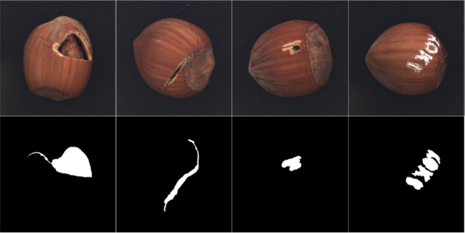
3. Network Architect
Our model had two main parts the Encoder and the Decoder. Each one had several convolutional layers followed by Batch-Normalization with 0.1 momentum and ϵ = 10−6 . For the activation function, we used the LeakyReLU with negative slope 0.01.3.1 Encoder Architect
Table 1 shows each layer and its dimensions for the Encoder.| LAYER TYPE | IN | OUT | KERNEL | STRIDE |
| CONV2D | 3 | 3 | 4 | 2 |
| BATCHNORM2D, LEAKYRELU | 3 | |||
| CONV2D | 3 | 32 | 4 | 2 |
| BATCHNORM2D, LEAKYRELU | 32 | |||
| CONV2D | 32 | 32 | 4 | 2 |
| BATCHNORM2D, LEAKYRELU | 32 | |||
| CONV2D | 32 | 32 | 3 | 1 |
| BATCHNORM2D, LEAKYRELU | 32 | |||
| CONV2D | 32 | 64 | 4 | 2 |
| BATCHNORM2D, LEAKYRELU | 64 | |||
| CONV2D | 64 | 64 | 3 | 1 |
| BATCHNORM2D, LEAKYRELU | 64 | |||
| CONV2D | 64 | 128 | 4 | 2 |
| BATCHNORM2D, LEAKYRELU | 128 | |||
| CONV2D | 128 | 64 | 3 | 1 |
| BATCHNORM2D, LEAKYRELU | 64 | |||
| CONV2D | 64 | 32 | 3 | 1 |
| BATCHNORM2D, LEAKYRELU | 32 | |||
| CONV2D | 32 | 500 | 8 | 1 |
| BATCHNORM2D | 500 |
3.2 Decoder Architect
Table 2 shows each layer and its dimensions for the Dencoder.| LAYER TYPE | IN | OUT | KERNEL | STRIDE |
| CONVTRANSPOSE2D | 500 | 32 | 8 | 1 |
| BATCHNORM2D, LEAKYRELU | 32 | |||
| CONVTRANSPOSE2D | 32 | 64 | 3 | 1 |
| BATCHNORM2D, LEAKYRELU | 64 | |||
| CONVTRANSPOSE2D | 64 | 128 | 3 | 1 |
| BATCHNORM2D, LEAKYRELU | 128 | |||
| CONVTRANSPOSE2D | 128 | 64 | 4 | 2 |
| BATCHNORM2D, LEAKYRELU | 64 | |||
| CONVTRANSPOSE2D | 64 | 64 | 3 | 1 |
| BATCHNORM2D, LEAKYRELU | 64 | |||
| CONVTRANSPOSE2D | 64 | 32 | 4 | 2 |
| BATCHNORM2D, LEAKYRELU | 32 | |||
| CONVTRANSPOSE2D | 32 | 32 | 3 | 1 |
| BATCHNORM2D, LEAKYRELU | 32 | |||
| CONVTRANSPOSE2D | 32 | 3 | 4 | 2 |
| BATCHNORM2D, LEAKYRELU | 64 | |||
| CONVTRANSPOSE2D | 3 | 3 | 4 | 2 |
4. Experiments
4.1 Training
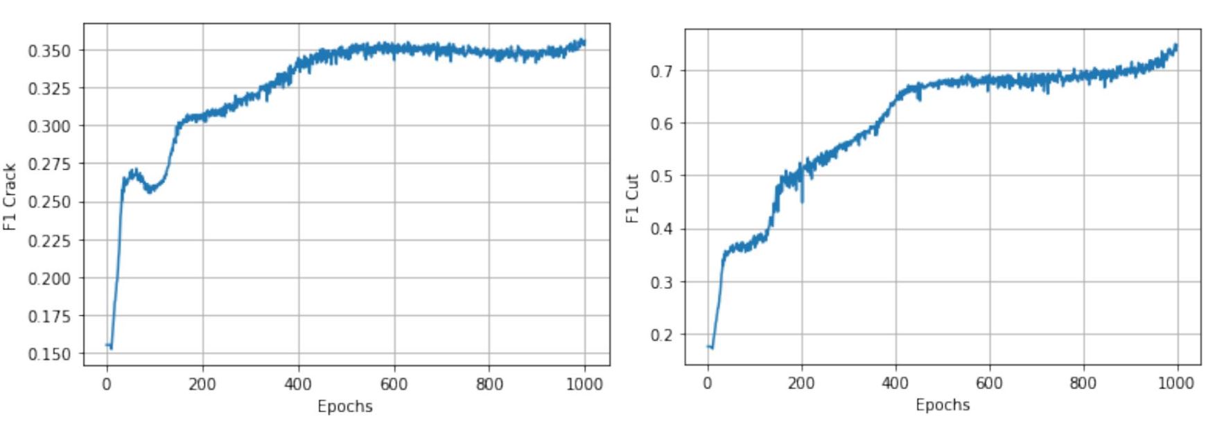
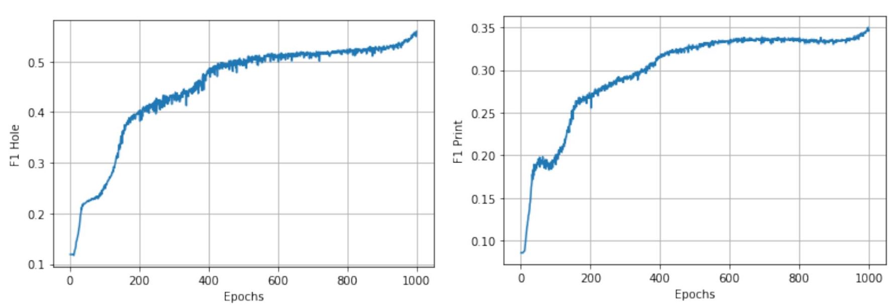
The model has been trained over the mentioned dataset for 1000 epochs. We used the ``L2`` loss for training our network using the ADAM optimizer. Figure 5 shows the loss for each step (each epoch has approximately 63 steps).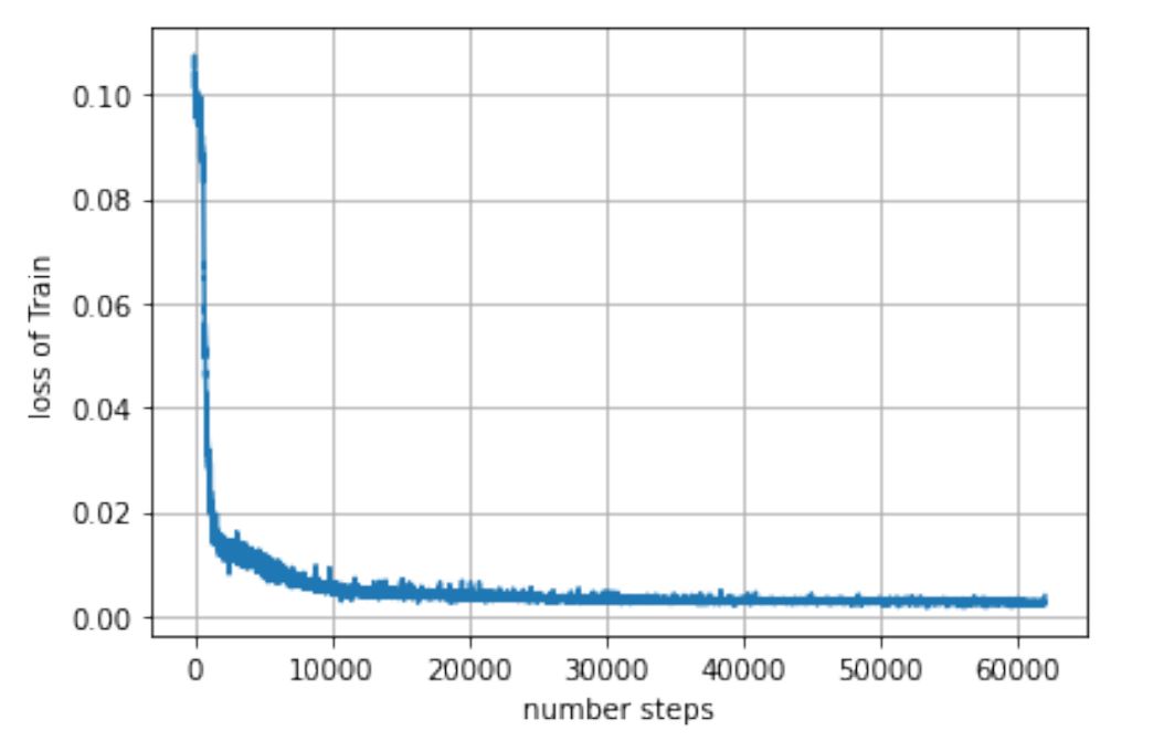
4.2 Methodology
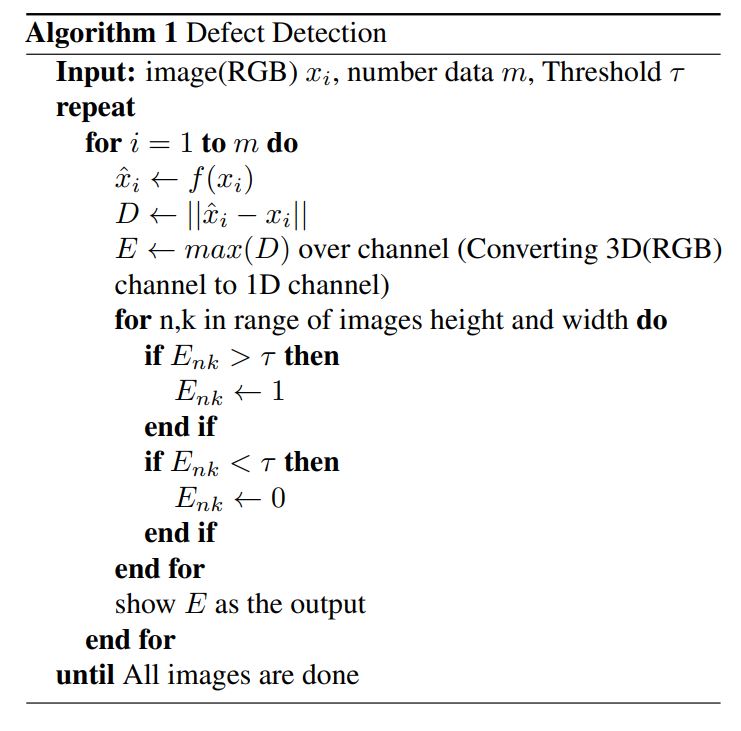
We are going to train our network to reconstruct the input image from the latent space. We do that by feeding many normal images to the network so the network will learn the distribution of standard and defect-free images. Since the latent space is smaller than the size of the image, the network learns the essential components of the image. After that, since it has learned the critical part, whenever it sees a new image, it will try to use the things it learned to construct the image. Since a defective image has regions that deviate from its distribution, it will have a high constructed error (difference between the input and output), and by that, we find the defective pixels.- Training: Input normal data to learn latent representation (Encoder). Use the latent representation to reconstruct the first image (Decoder).
- Testing: An image with a defect will have a different output compared to the expected input. Hence errors will be high. Apply a threshold for the reconstruction error to detect the error.
4.3 Outputs
We used the algorithm to detect the defect in the testing images, and for every dataset, here is the result. From left to right Original Image, Output Image, Predicted Pixels, Ground Truth.- Crack:
- Cut:
- Hole:
- Print:


5. Discussions
5.1 Effect of Threshold
The output depends on the parameter τ. In figures 13 and 14, the effect of the threshold can be seen. If the threshold value is too high (for example, τ = 0.7 in figure 14), the system will miss some defective pixels. Therefore the F1 accuracy will decrease. If the threshold value is too low (for example, τ = 0.1 in figure 14), the system will assume that the defect-free pixels are also defective. In this case, the F1 will also decrease since many pixels do not contain faulty pixels, but the system will predict it anyway.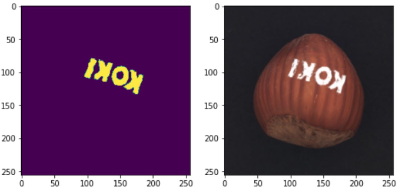

5.2 Effect of Latent Space size
In our model and result, the dimension of the latent space was 500. However, this is a hyper-parameter that we could change. Changing this parameter will cause effects on the output. As we mentioned, Decoder's objective is to reconstruct the input data from the output of the Encoder (aks the latent vector). If the latent size space is too small, the model will face difficulties learning small details since it has less power to learn the latent space distribution. Therefore in some cases, it is likely that some pixels have defected while they are entirely defect-free. If the latent space is too large, the model will start to memorize the input image instead of learning the image features. The model is likely to construct an image that has the same defective parts. This might lead to a situation that the model is not able to detect the faulty pixels in an image.In the last part, we are going to compare our results with other methods and approaches that are out there.
6. Conclusions
In the last part, we are going to compare our results with other methods and approaches that are out there.
| METHODS | RECALL | PRECISION | F1 |
| OUR METHOD (PRINT) | 0.22 | 0.82 | 0.35 |
| OUR METHOD (CRACK) | 0.26 | 0.57 | 0.36 |
| OUR METHOD (CUT) | 0.69 | 0.8 | 0.57 |
| OUR METHOD (HOLE) | 0.55 | 0.61 | 0.75 |
| AE(SSIM) | 0.08 | 1 | 0.15 |
| AE(L2) | 0.84 | 0.93 | 0.88 |
| ANOGAN | 0.16 | 0.83 | 0.27 |
| CNN FEATURE DICTIONARY | 0.07 | 0.9 | 0.13 |
We compared our approach with some of the models that are already used and it seems Paul Bergmann, January 2021 has the best performance when they train their model on an L2 loss function. But it seems that our approach is good since we outperform other methods such as AnoGANs, Auto Encoders using SSIM and CNN feature Dictionary. However, our approach has a lower accuracy in all 3 metrics (Recall, Precision and F1) compared to the state-of-the-art method. In one special case, the AE approach with the SSIM loss function was able to reach 100 % for precision, however, they were not able to have a good performance of the Recall, therefor according to our F1 metric, our approach outperforms the AE(SSIM) approach.