Image-to-Image Translation (CycleGAN)
Disclaimer
I tried to reproduce the results from Unpaired Image-to-Image Translation using Cycle-Consistent Adversarial Networks (project link). I had no contribution over the original paper, all I did was to recreate the same results from the paper.Abstract
Image-to-image translation is one of the tasks in deep learning that has gotten a lot of attention in the deep learning and computer vision community. However, in the more traditional approaches, there must be labelled images for corresponding images, e.g. for every image from domain A there must be an image B in the other domain. However, in the approach that Jun-Yan Zhu et el, they did not need the corresponding images from the two domains.
1. Introduction
1.1 Paired Data
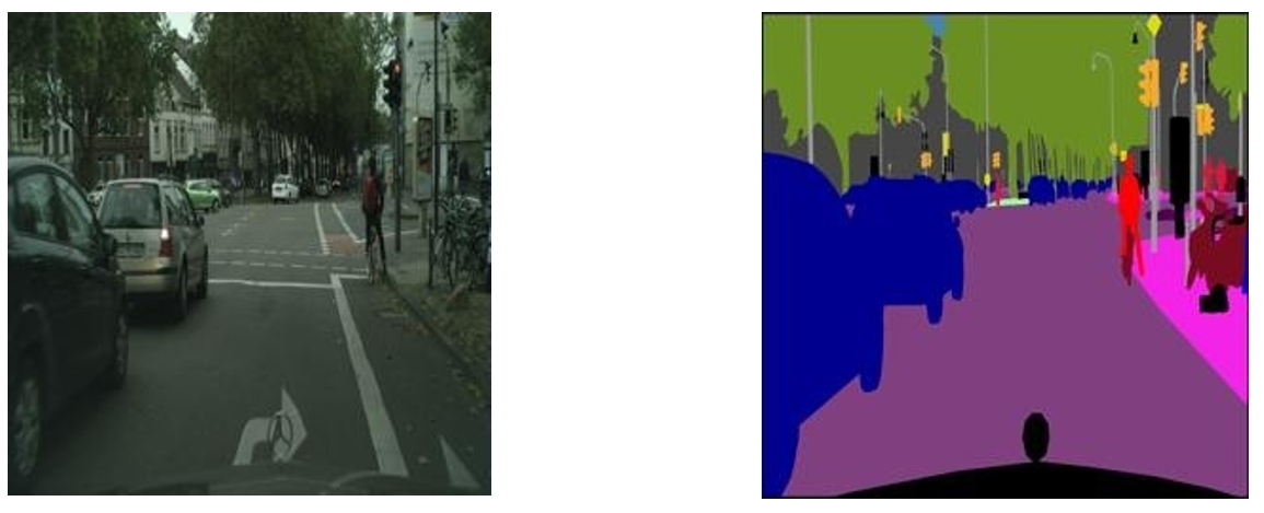
In image-to-image translation tasks, one important thing is the need for paired data. Figure 1 shows an example of paired data. However, there are limited datasets that have paired data. But CycleGAN introduces a new method to the image-to-image translation task without paired data. This is a significant boost in the field of image-to-image translation.
1.2 Adversarial training
Figure 2(a) shows the entire model, where we indicate that domain `X` is the real image and domain `Y` is the segmentation domain. Model `G` is a generator that converts images from domain `X` to domain `Y`, in other words, `G:X\rightarrow Y`. Model `F` is a generator that converts images from domain `Y` to domain `X`, in other words, `F:Y\rightarrow X`. There are also two discriminators whose objective is to detect whether the input image is real or fake. Discriminators `D_{X}` will detect whether the ground image (the real image from the scene) is real. Discriminators `D_{Y}` will detect whether the segmentation is real.

1.3 Cycle Consistency
Adversarial training can, in theory, learn mappings `G` and `F` that produce outputs identically distributed as target domains `Y` and `X,` respectively. However, with a large enough capacity, a network can map the same input images to any random permutation of images in the target domain, where any of the learned mappings can induce an output distribution that matches the target distribution. Thus, adversarial losses alone cannot guarantee that the learned function can map an individual input `x_i` to a desired output `y_i.` The learned mapping functions should be cycle-consistent to reduce the space of possible mapping functions. Figure 2(a) shows the concept of cycle consistency. In this (cycle consistency) approach, after applying generator `G` to an image, we will also apply the function `F`, which will convert `G(X)` back to domain `Y`. The overall goal is to make `X` and `F(G(X))` as close as possible. We also do the same thing reversely, where the goal is to make `Y` and `G(F(Y))` as close as possible.
1.4 Identity loss
Besides the two methods we just mentioned, they also used one additional loss to train their model. If we apply generator `G` to an image that is in domain `X,` we expect it to stay in the same domain, which means `G(X)=X.` The opposite should also work, which means if we apply generator `F` to an image from domain `Y,` it should remain in domain `Y.` Figure 3 shows this concept.


2. Dataset
We used the Cityscape dataset, which contains images and their corresponding segmentation. Figure 1 shows a sample of these images.
3. Network Architecture
We used Johnson et al model since Johnson et al were able to achieve impressive results for neural style transfer and super-resolution. The network contains three convolutions, several residual blocks, two fractionally-strided convolutions with stride 0.5, and one convolution that maps features to RGB. They use 6 blocks for 128 × 128 images and 9 blocks for 256×256 and higher-resolution training images. They also used instance normalization in their model. For the discriminator networks, they used 70 × 70 PatchGAN which aims to classify whether 70 × 70 overlapping image patches are real or fake.
4. Training
We trained the model using a pre-trained model(trained on a different dataset), with a learning rate of 0.0002. We divided the objective (loss) by 2 while optimizing `D`, which slows down the rate at which `D` learns relative to the rate of `G`. They kept the same learning rate for the first 100 epochs and linearly decayed the rate to zero over the following 100 epochs. Weights are initialized from a Gaussian distribution `N(0, 0.02)`.
4.1 Discriminator loss
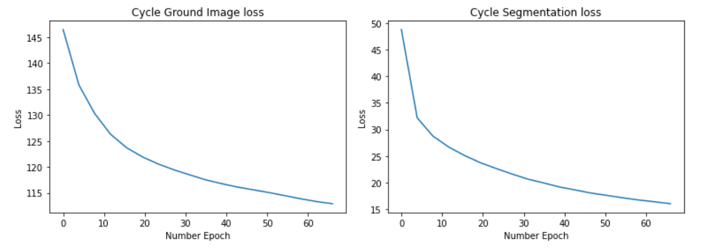
4.2 Cycle Consistency loss
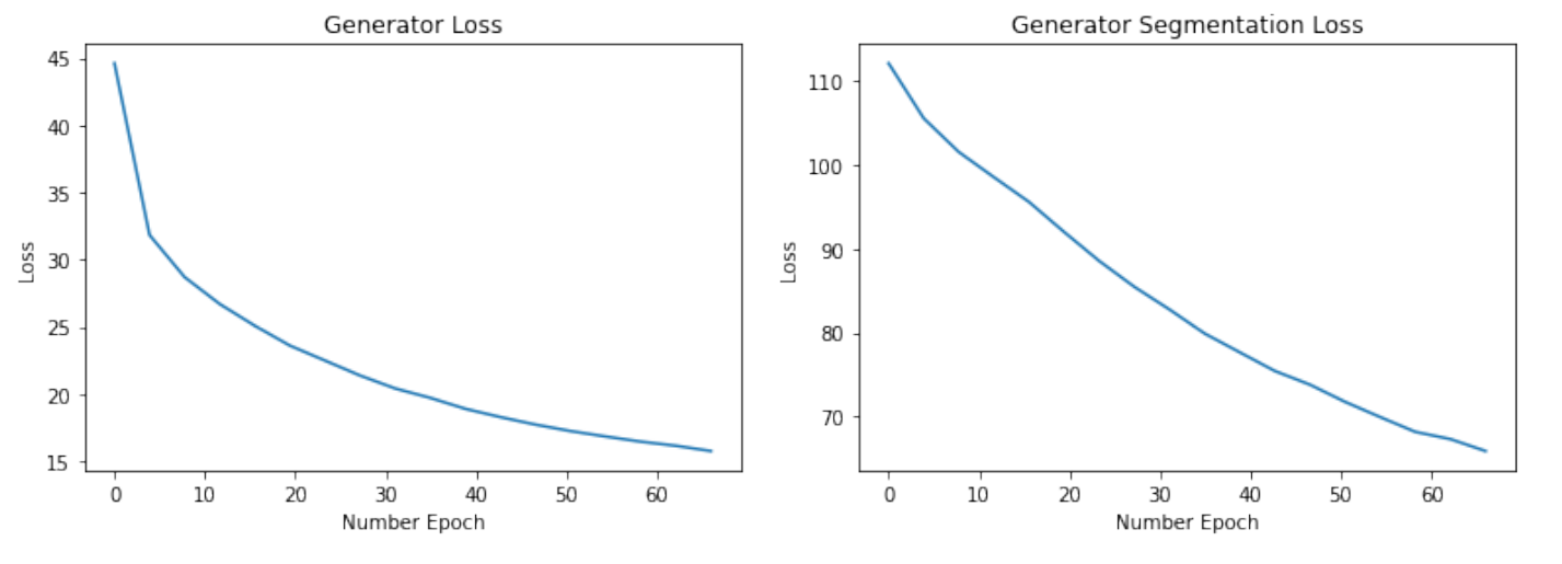
4.3 Generator loss
4.4 Discriminator Accuracy
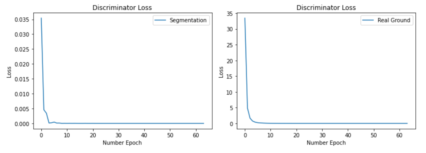
We trained our model for 200 epochs. Figure 7 shows the accuracy of the discriminator, where it shows the percentage of correct guesses for the discriminator for detecting real ground images or fake ground images.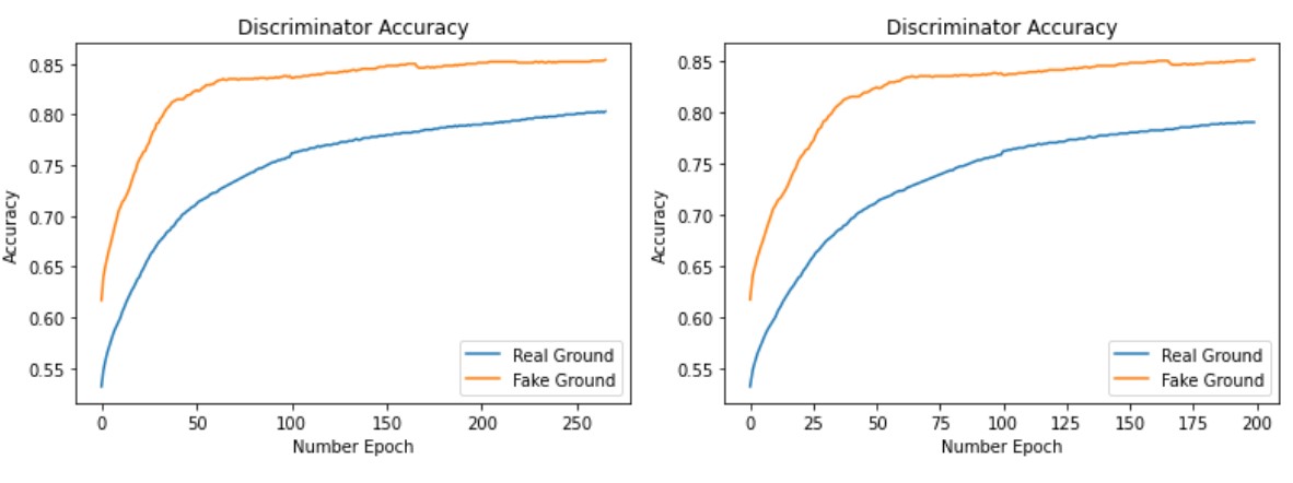
5. Results
We conducted two different experiments 1. We only used the cycle consistency loss 2. In addition to the cycle consistency loss, we used identity loss. In the second case, we assumed that ` \lambda_{C} = \lambda_{I}`. Where `\lambda_{C}` is the coefficient of cycle consistency loss, and `\lambda_{I}` is the coefficient of identity loss.5.1 Cycle Consistency Loss Only
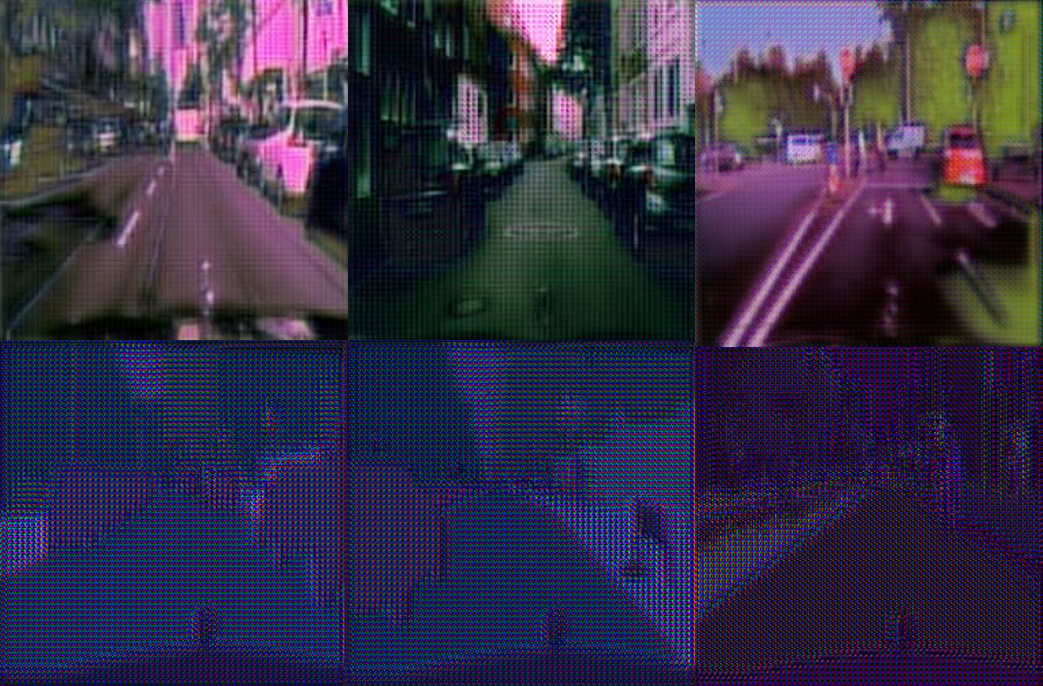
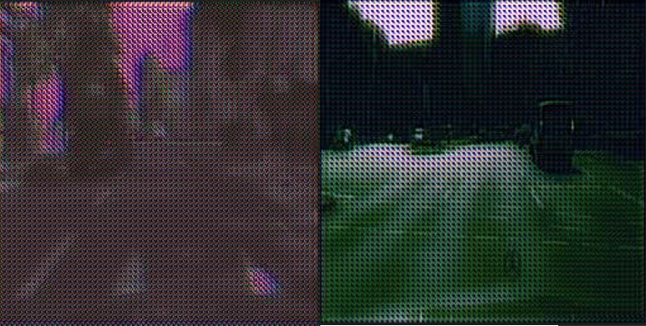
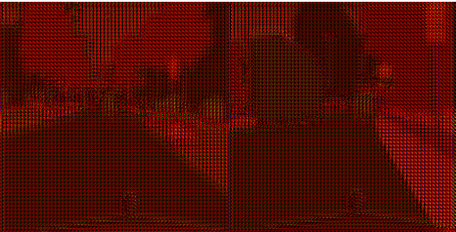
We trained our model for 200 epochs. Figure 7(left) shows the accuracy of the discriminator, where it shows the percentage of correct guesses for the discriminator for detecting real ground images of fake ground images. Our results and output were quite reasonable; however, we could not train the entire model to its full potential due to our limited resources. The results were not bad. The performance for generating ground images was better. Figure 8 & Figure 9 shows the result of our CycleGAN after 200 epochs of training without applying the identity loss.
5.2 Cycle Consistency Loss + Identity Loss
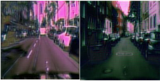
Since we had limited access to Google Colab servers, we used the weights from the previous model instead of just re-training our model (the model with no Identity loss). We fine-tuned the model with the new hyper-parameters. The only difference in the two hyper-parameters is that in the case we used the identity loss, parameter `\lambda_{I}` was not 0 and was the same value as `\lambda_(C)`. We trained our model for another 70 epochs, and figure 7(right) shows the model's accuracy during training. This accuracy indicates the number of times the model has detected if the image was real or fake. Since we were fine-tuning the model, the first 200 epochs are the same as in figure figure 7(right). The final result from fine-tuning the model is in figure 10 and figure 11. We can see the significant improvement in the ground image result in figure figure 10. Meanwhile, the result for the segmentation model in figure 11 did not show much improvement.
6. Conclusion
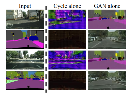
To sum up, the result we got from this project was not the exact same as the main paper itself. However, the results were quite acceptable. By looking at the generated images, we could see that the model's performance over generated ground images is quite well, but of course not as good as the main images. The results of the generated segmentation images were not as good as the ground images. One thing that we need to consider is that every colour in the segmentation image is going to represent a particular class. However, what the CycleGAN model sees is a normal image, and it will treat the image the same way, which is why the segmentation results are not categorized. Since the segmentation output is not categorized(the output was just an RGB image), we could not fully reconstruct that part. It is also interesting since in the paper in (look at figure figure 12) they showed the result they had when they used Cycle Alone is quite similar to the result that we have gotten in our implementation. However, their final result is better than ours.
